By R. Austria, M. Gutierrez, F. Luces
Very popular pre-2000, when computer processing bandwidth was at a premium and engineers had more time to put together study information on the desktop (the wooden one, not the one filled with integrated circuits), equivalencing appears to have gone the way of the calculator, the clock and the calendar. Ok, so not quite, as the smartphone does not yet have an “equivalent” function. This will have to wait until analytical programs for power system analysis are made portable. But nonetheless, today’s power engineers will more readily go for the brute force approach of “model everything” rather than take the extra time and effort of creating a simplified model.
However, there remain many situations where equivalencing has value to power system analysis. Examples:
- Numerical issues. Software for bread-and-butter analysis such as power flows, dynamic simulation and transient analysis are still founded on iterative methods. The larger the power system, the larger the model (in terms of number of elements), and small numerical issues become big numerical issues; e.g., non-convergence and divergence, error accumulation and drift, non-linearity, etc.
- Modeling issues. Large databases are frequently contributed to by multiple entities with varying degrees of accuracy, diligence, application of standards and maintenance. These databases are a hodgepodge of components connected only at the seams and largely unregulated.
- Local issues. There are two aspects to this. One, most power system issues tend to be localized in nature; i.e., an overload in New York is not likely to influence what’s going on in Florida. (This is not to stay that all such issues are local, as an issue such as inter-area dynamic oscillation clearly affects a broad region if not the totality of a model.) Two, a modeling or numerical issue can start small and very localized but eventually affect the whole analysis. For example, voltage collapse may initiate at a specific location’s lack of reactive power but then propagate farther out as more and more reactive sources are drawn upon.
Furthermore, to some degree, all databases use equivalents of one form or the other. Let’s start with some basics.
What are equivalents?
An equivalent represents a small portion of the grid for the purposes of studying local conditions, where, as noted earlier, a small portion could mean the whole state of New York or the Northeast United States, or Michigan. In this context, an equivalent is an artificial group of branches and buses that represents the behavior of the external system as seen from its boundary buses (see figure).
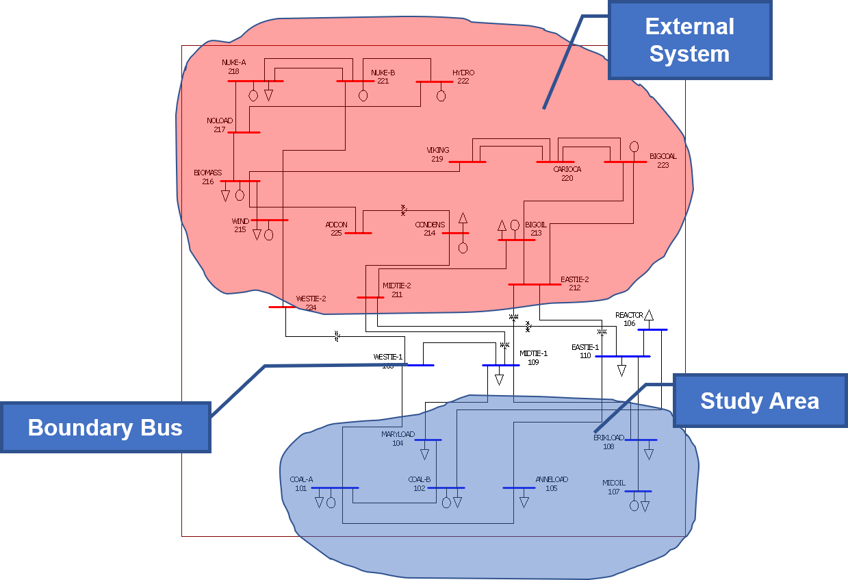 In this example, the area to be equivalenced is the external system. The number of boundary buses and retained buses determines the number of equivalent branches. Retained buses are selected non-boundary buses that may have a bearing on the equivalent.
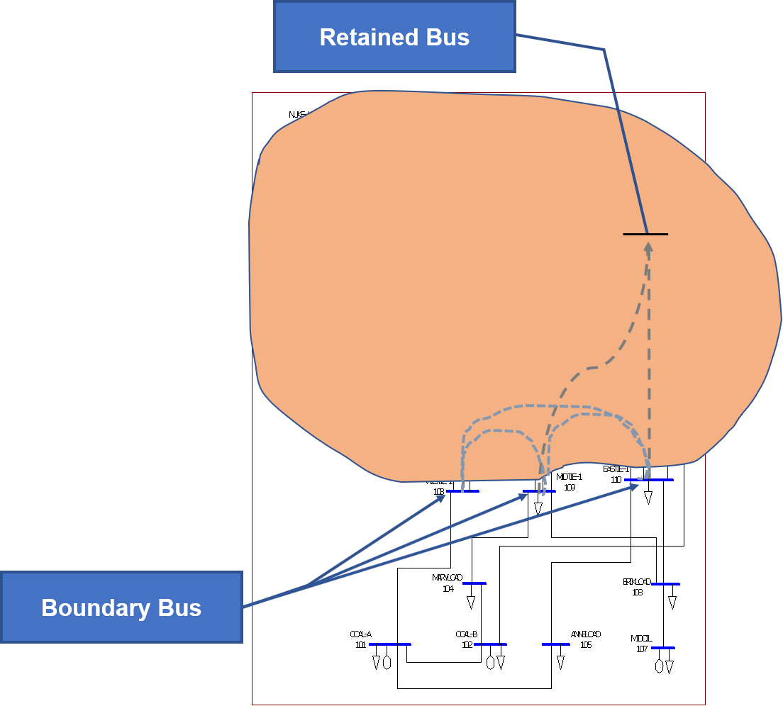
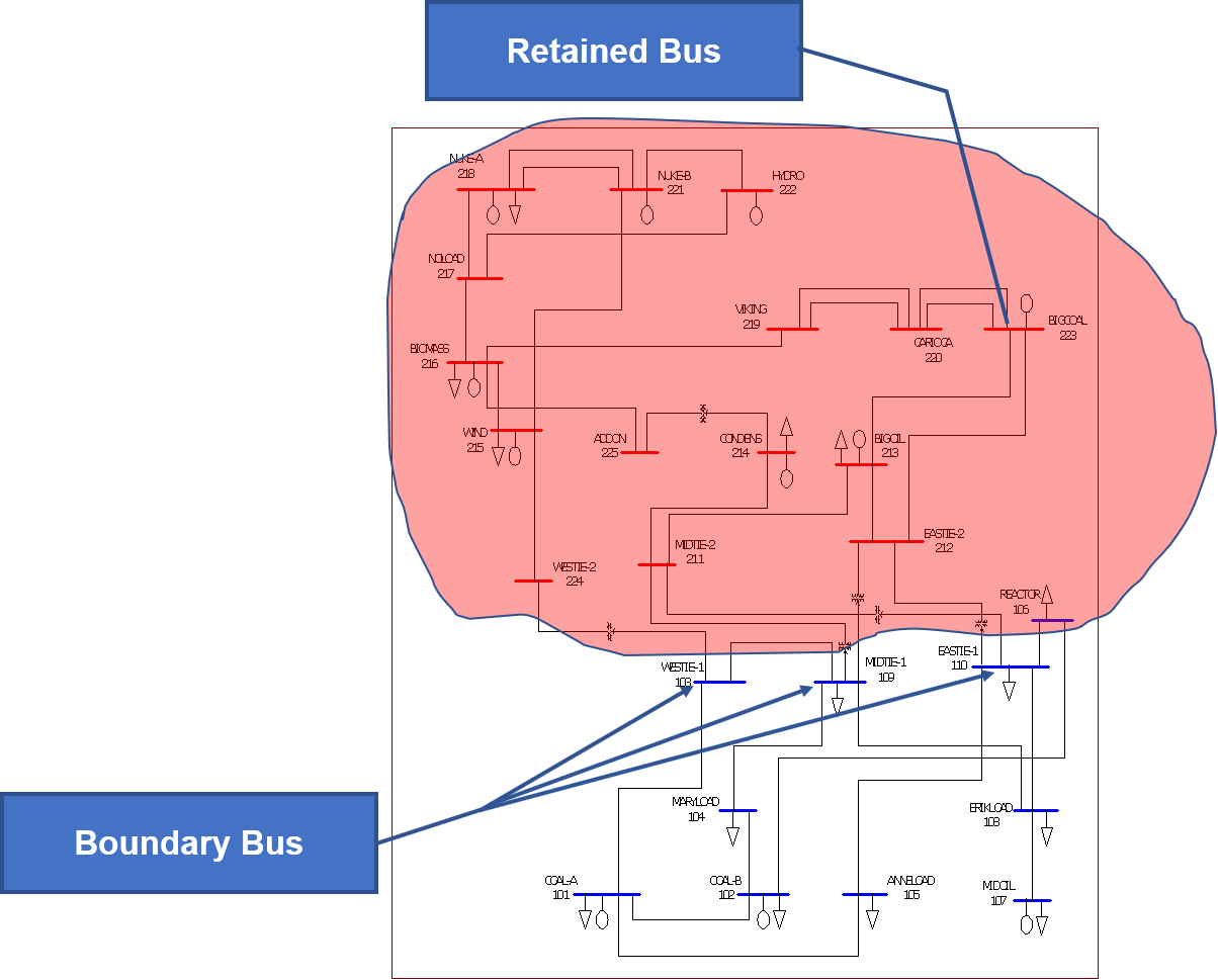 The number of boundary buses and retained buses determines the number of equivalent branches. Large impedance branches can be excluded from equivalent as they represent a path that will resist or “impede” power flows, and therefore, will not figure significantly in the power flow solution except in the matter of convergence.
 There are several forms of equivalents intended for different purposes. For power system studies, we are interested in:
- Power Flow equivalents
- Short circuit equivalents
- Dynamic equivalents
The Power Flow Equivalent
Given a power flow case defined by the matrix equation:
![\[\left[\begin{matrix}I_a\\I_b\\\end{matrix}\right]=\left[\begin{matrix}Y_{aa}&Y_{ab}\\Y_{ba}&Y_{bb}\\\end{matrix}\right]\left[\begin{matrix}V_a\\V_b\\\end{matrix}\right]\]](https://www.pterra.com/wp-content/ql-cache/quicklatex.com-d4c2ea9609f622bb742838873b66fc3a_l3.png "Rendered by QuickLaTeX.com")
Where  and
and  are node current and voltage at the nodes to be retained, and
  and
and  are node current and voltage at the nodes to be deleted.
The matrix can be reduced using Gaussian elimination or Kron’s Reduction method to produce:
![\[I_a=\left(Y_{aa}-Y_{ab}Y_{bb}^{-1}Y_{ba}\right)V_a+Y_{ab}Y_{bb}^{-1}I_b\]](https://www.pterra.com/wp-content/ql-cache/quicklatex.com-921b7bb851737678791b97f9421ade23_l3.png "Rendered by QuickLaTeX.com")
The first term defines the relationship between the voltage and current among the retained nodes. The second term defines the current superimposed on retained nodes to reflect the effect of the deleted nodes. These imposed currents are precise with respect to the original whole database but become approximate when changes are made to the study area. The key aspects to consider are:
- Are the boundary buses sufficiently far from the focus of study to capture all the local effects without significant degradation in accuracy of the model? Sometimes including some large external generators via retained buses can be helpful.
- The accuracy of the equivalent will also depend on the size of the system to be equivalenced, represented by
 . Since the formula given above is linear, it is possible to apply it multiple times, e.g., do small bites of the external system until the whole external system is equivalenced.
Also, note that once equivalenced, most of the information on the external system is lost so that it is not possible to recover the full system from its equivalent.
Short Circuit Equivalent
For short circuit analysis, generators are modeled as Norton equivalents. The “equivalent” in this context refers to the balance of plant as seen from the generator terminals or point of interconnection with the grid. In fact, large scale power system models are replete with these “internal” equivalents, primarily lower voltage systems that are represented by some model as seen from a node in the grid model. This includes substation loads, reactive supply equipment, substation lower voltage system, collector systems for wind and solar farms and large-scale batteries, and so on. With increasing computing capability, it might one day be possible to include these lower voltage components into an even larger and more-encompassing database model. With that would come, hopefully, improvements in the solution methods such as knowledge networks, self-correcting and self-learning algorithms and so on.
Anyway, short circuits are also a localizable phenomenon, and quite amenable to the form of large-scale system model equivalencing we have thus far been discussing. To obtain such as equivalent, replace the currents and in the previous equation with the generator Norton-source currents.
Note that since unbalanced conditions may be present in short circuit analysis, it may be necessary to develop coordinated equivalents of the positive, negative and zero sequence portions of the network. Generally, this means that the retained and boundary nodes be coincident amongst the sequence models. The positive, negative and zero admittances for the same element are different.
It is interesting to note that the fault level (the result of a short circuit calculation) at a specific node is in itself an equivalent of the network as seen from that node.
![\[I_{sc}=\frac{V_{Th}}{Z_{Th}}\]](https://www.pterra.com/wp-content/ql-cache/quicklatex.com-b8ba05c5c9fb95f3a0650132a5ef1988_l3.png "Rendered by QuickLaTeX.com")
Where  is the short circuit current at a node,
  is the Thevenin equivalent voltage as seen at the node, and
  is the Thevenin equivalent impedance as seen from the node.
In contradiction to what was said earlier in the power flow section, it is possible to build up the equivalent comprising of several nodes from the fault level of each of the nodes. Take the case of two nodes, 1 and 2, connected by a transformer.
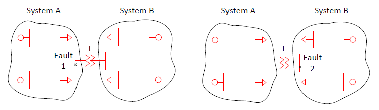 The fault level at each side of the transformer is known (at locations 1 and 2), as is the impedance of the transformer itself. Assuming is 1.0, then
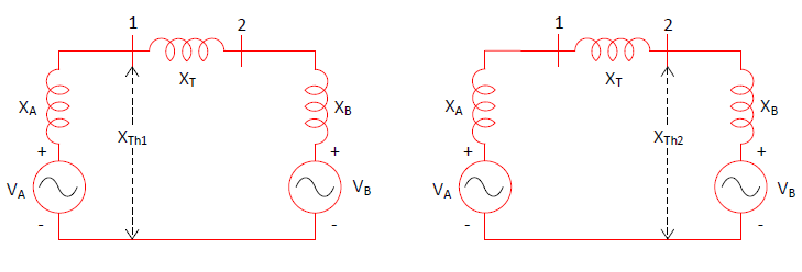
![\[{MVA}_{SC1}=\frac{{MVA}_{Base}}{X_{Th1}}\]](https://www.pterra.com/wp-content/ql-cache/quicklatex.com-1294c00c0fffb31482356d44fd0fda55_l3.png "Rendered by QuickLaTeX.com")
![\[{MVA}_{SC2}=\frac{{MVA}_{Base}}{X_{Th2}}\]](https://www.pterra.com/wp-content/ql-cache/quicklatex.com-d54670dca95b18464c4114ae71a47825_l3.png "Rendered by QuickLaTeX.com")
Where
![\[X_{Th1}=\frac{X_A\left(X_T+X_B\right)}{X_A+X_T+X_B}\]](https://www.pterra.com/wp-content/ql-cache/quicklatex.com-4721bc46782f08ddd5b426d5826262eb_l3.png "Rendered by QuickLaTeX.com")
and
![\[X_{Th2}=\frac{X_B\left(X_T+X_A\right)}{X_A+X_T+X_B}\]](https://www.pterra.com/wp-content/ql-cache/quicklatex.com-aca068c9b6a8860f9a4aded71f944047_l3.png "Rendered by QuickLaTeX.com")
From which, the values of  and
and  can be obtained. We now have a 3-node equivalent developed from the fault levels of two nodes. If we have a third node whose fault level is known, we can add another node to the equivalent, and from there construct even higher dimensioned equivalents with further values of fault levels.
Dynamic Equivalent
For dynamic simulation, control models are added to the power flow database. Typically, these comprise of generator dynamic response for electromechanical interaction (for rotating machines), photovoltaic conversion (for solar farms), voltage/reactive power control and frequency/speed control. In addition, specialized equipment such as static VAR compensators, high-voltage direct current transmission lines, protective relays, among others, may be included in the database.
There are various methods for creating a dynamic equivalent. A simple one, but quite adequate for most purposes, follows:
- Create a short circuit equivalent, using the sub-transient value of impedance to model the Norton generators.
- Create a power flow equivalent, coincident with the short circuit model, to obtain the size of the equivalent load and generation at each boundary and retained bus.
- Add the generation and load from the power flow equivalent at the boundary and retained buses of the positive sequence short circuit equivalent.
- Add dynamic models for the generators and loads at the boundary and retained buses. If the boundary buses are sufficiently far from the study, a classical generator model with constant flux may be applied. Otherwise, use generic models for the generator energy conversion dynamics and any associated voltage and frequency controls.
- To ensure equivalent performance, run test disturbances with the full system and the equivalenced system to tune the generic models.
There are, of course, much fancier approaches that are available in the literature. See for example:
- Podmore, R. Dynamic equivalents for transient stability studies of very large synchronous networks. Final report. United States: N. p., 1979. Web.
- Bree, D & W. deMello, R & C. Markel, L & N. Stanton, K & A. Walker, R. (1974). Coherency based dynamic equivalents for transient stability studies. PICA Conference Proceedings.
- P. Accari, W. W. Price, J. H. Chow, R. Galarza. Inertial and Slow Coherency Aggregation Algorithms for Power System Dynamic Model Reduction, IEEE Transactions on Power Systems, Vol. 10, No. 2, May 1995.
Closing Notes
There remain many opportunities for applying equivalencing in power system analysis. While commercial software continue to use single path numerical methods for solutions, the issue of non-convergence and divergence remain. The issue of drift in simulations will expand as explicit integration is the prevalent method for power system dynamic simulation. And the issue of uneven quality of models in a large-scale database will be present while there is no extensive standardized modeling practice.
Equivalencing remains good industry practice, and an important skill for power system engineers.