(A serialized and expanded version of this article can be found here)
As an increasing number of wind turbines are connected to the power system, more and more wind farm interconnection studies are requested. Usually a wind farm consists of tens of wind turbines and cables. The wind turbines are mostly the same type in one particular wind farm, but the cables interconnecting these wind turbines vary in length, capacity and configuration. A transmission analyst may need to avoid modeling each turbine and each cable in the wind farm for the interconnection study for one or more of several possible reasons:
- It is laborious to setup the detailed model. For example, a 300 MW wind farm would comprise of 200 1.5-MW wind turbines interconnected at a distribution level voltage such as 34.5 kV in a feeder network similar to that of a suburban housing development. The simulation software for power flow, short circuit or stability analysis may not accommodate carrying detailed models for all the existing and proposed wind farms. To consider the dimensions, take the case of a system with some 5000 MW of installed wind capacity. Detailed modeling of the wind farms would require about 4000 turbine models, 5000 additional nodes and the same number of additional branches in the database.
- The detailed model requires representation of distribution level feeder circuits that increase the “spread” of branch impedances in the power flow model. “Spread” here refers to the range of impedances included in the database. (see further discussion about spread or diversity in the article, “Converging the Power Flow”). Too much spread can lead to difficulties in solving, or converging, the power flow.
In view of all the above reasons, it may be sufficient to aggregate groups of wind turbines into equivalents that capture their net impact on the transmission system.
Modeling Issues
For a typical interconnection study consisting of power flow calculation, transient stability and short circuit analysis, the aggregated wind farm model must effectively represent the behavior of the wind farm during
- steady-state operation;
- switching operations or short circuit occurrences;
- transient period following planned and unplanned events such as a fault, line trip, breaker reclose, or trip of a turbine.
The components that need to be considered in the aggregate modeling are:
- Steady-state, short circuit and stability models of the individual turbines. Typically, a farm will use the same type and manufacture of wind turbine throughout. Aggregating the individual turbines is straight-forward in this case. Most turbine models have the characteristics of aggregating by capacity. For example, GE1.5 wind turbine generator model variables are in per unit on the generator MVA base. To model the aggregated unit, only the generator MVA base need be changed to the sum of the individual turbine MVAs. If the turbines are of different types (for types of wind turbines, please see article on Wind Farms), a more involved process for aggregating is required to obtain a good equivalent. In general, interconnection studies assume that each turbine sees the same wind speed; however, in reality, the wind diversity across a farm is such that some turbines may be below the wind threshold and delivering zero power while others may be at full power.
- Electrical layout of a wind farm. The layout of a wind farm looks much like a suburban housing development where the “houses” or in this case, the individual wind turbines, are spread out to minimize wind shadows and maximize wind capture. The turbines are interconnected by feeders that are arranged and optimized similar to a suburban distribution network, only in this case, they are part of the “collector” system. The more wind turbines there are in the farm, the more complex the collector system. For aggregation purposes, if the feeder is radial, one aggregate may be developed for the whole feeder, as shown in Figure 1. For the electrical impedance of the equivalent feeder, the two most common practices are: (a) use the sum of the feeder impedance to the farthest wind turbine or (b) use a rule-of-thumb for the equivalent impedance to be 1/3 of the total feeder impedance.
- Step-up transformer characteristics. These are generally modeled explicitly, even if the wind turbines are aggregated.
- Capacitor banks and static var devices. These are also modeled explicitly.
Figure 1A shows a detailed wind farm with 16 turbines arranged in two radial feeders, and in Figure 1B, a proposed equivalent with two aggregates, one for each feeder. In the figure, the numbers in the circles represent the total number of turbines at the corresponding buses. In the detailed model, each turbine is modeled exactly as it is electrically located in the wind farm, and each wind turbine bus has only one turbine connected. In the simplified model, two aggregated wind turbines are modeled at the remote end of each cable branch, one lumps together twelve wind turbines and the other, four wind turbines.
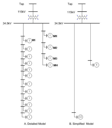
Figure 1: (A) Detailed Wind Farm Model and its (B)
Simplified Equivalent
For steady state analysis, the two models show very similar performance characteristics. Actually, the difference between these two models comes from some minor power loss differences on the cables connecting the wind turbines. Since in the steady state analysis, the wind farm is modeled as seen from the system, only the effects of the power injection into the system are considered while the internal wind farm behavior is neglected.
For transient stability analysis, the aggregated model closely represents the wind farm especially when the cables connecting the wind turbines are short. However, there are cases where the internal wind farm responses are different, and these result in significant differences in impacts on the system.
For short circuit analysis, the two models’ differences in the interconnection study vary. For those wind turbines that do not contribute short circuit current , the modeling choice does not matter. For example, Clipper’s permanent magnet wind turbine generator has no shirt circuit current contribution. For those wind turbines that contribute short circuit current, the detailed model might have higher current than that of the simplified model.
Test Case
In our test case, a wind farm, sized 32MW and shown in Figure 1(A), is proposed for interconnection to an existing 115 kV line rated 105 MVA. In the simplified model, the feeder branches are modeled with full equivalent impedances, i.e. the corresponding largest impedance of the feeder.
- Performance in the steady-state: The power injections at POI (point of interconnection) for the detailed model and simplified model are 31.6MW and 31.5MW respectively, and the corresponding reactive demands and voltages at the POI are 0.7MVAR, 1.020p.u. and 0.2MVAR, 1.022p.u., respectively. The active and reactive power differences are due to the minor power loss and voltage profile differences on the interconnecting cables. The difference in power delivered at the 115 kV POI constitute less than 1% of the line rating and will not have a significant impact on the steady-state thermal performance. The 0.5MVAR difference in reactive power demand likewise will not significantly change the steady-state voltage performance of the models. (The farm is small enough that it may be interconnected to a 69 or 34.5 kV system. If this is the case, the thermal and voltage impacts from the difference in modeling can be more significant.)
- Short circuit performance. For this test case, the wind turbine generator has no short circuit contribution. As such, the maximum fault current level with the addition of the wind project will not change.
- Transient stability performance. The models show very similar performance for most disturbance except for those close to the POI. When a three-phase fault is applied at the POI, the terminal voltage of the wind turbine next to the step-up transformer in the detailed model (at units marked as “N1” and “M1” shown in Figure 1A) is less than that of the corresponding aggregated turbine in the simplified model. The voltage difference might cause the situation that some wind turbines in the detailed model are tripped due to low voltages while the aggregated turbines in the simplified model are all online. Figure 2 shows simulation results for the test case for a 3 phase fault at the POI, (A) for the detailed model and (B) for the simplified or aggregated model. In Figure 2, the active power (pbr), current (ibr) through the transformer and the voltage (vbus) on the low side of the transformer are monitored. In the detailed model case, the four turbines on the right branch (units “M1” to “M4”in Figure 1) are all tripped due to low voltages, while the aggregated turbines in the simplified model all stay online. The simulation of the detailed model shows that the terminal voltages for units “M1” to “M4” dip low enough and for long enough to trip the wind turbines’ voltage protection. On the other hand, the terminal voltages of the aggregated units are above the limits.
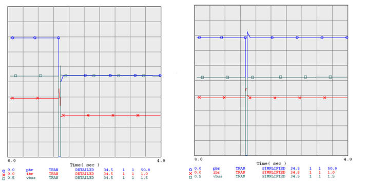
Figure 2: Different Responses of the (A) Detailed Model
and the (B) Simplified Model (Output from PSLF software; PSLF is a
commercial product of General Electric Energy)
For test purposes, a partial equivalent feeder impedance equal to 1/3 of the full impedance is applied to the simplified model. This model is more conservative with respect to the voltage profile during the fault than the model with the full equivalent impedance. Applying the same fault at the POI, with 1/3 of the corresponding maximum feeder impedance, the lumped unit with 4 turbines is tripped. This is a similar result to the case with detailed model.
Another observation of note in the test case: when re-dispatching involving the wind farm is required, it is easier switch on/off turbines in a detailed model than to calculate the new equivalent in the aggregated model.
Conclusions
- In general, an aggregated model provides a good enough approximation of the wind farm performance for use in interconnection studies.
- There are certain situations when a detailed model isrequired.
- When the size of the wind farm to be interconnected is significant relative to the network; for example, a 30 MW wind farm to a 34.5 kV network
- When the fault is applied at or close to the POI for transient stability performance
- To avoid inaccuracies, a detailed model is preferred when simulating close-in faults for transient stability. All other faults can be simulated with acceptable accuracy using a simplified model. When applied to interconnection studies, it is usually sufficient to model other wind farms which are not the subject of the assessment using a simplified model.
References
- J.G.Slootweg, W.L. Kling, “Aggregated Modeling of Wind Parks in Power System”, Power Engineering Society Summer Meeting, 2002 IEEE, Volume 1, 25-25 July 2002 Page(s):503 – 508 vol.1
- M. Poller, S. Achilles, “Aggregated Wind Park Models for Analyzing Power System Dynamics”, online: http://www.digsilent.de/Consulting/Publications
- K. Elkington, V. Knazkins, M. Ghandhar, “On the Rotor Angle Stability of Power Systems with Doubly Fed Induction Generators”, Power Tech, 2007 IEEE Lausanne, 1-5 July 2007 Page(s):213 – 218
- PSLF Users’ Manual, August, 2006
- Clipper Liberty Brochure.
© 2009. All rights reserved.